This section includes the following topics:
- About Precise for SAP tabs
- How most tabs are structured
- About drilling down in context
- About configuring Precise for SAP settings
- Tasks common to all tabs
- About the counters in Precise for SAP
- Launching your Precise product from StartPoint
About Precise for SAP tabs
Precise for SAP is a comprehensive performance management product for SAP. It provides specialized data collection and analysis capabilities of SAP Application Servers and it enables you to find performance and availability bottlenecks.
Precise for SAP contains the following tabs that provide you with the information necessary to successfully track your system’s performance and identify patterns in resource consumption.
The following table describes which tasks can be performed in each tab.
Table 1 Precise for SAP tabs
| Tab | Description |
|---|---|
| Dashboard | The Precise for SAP Dashboard is an easy-to-use tool for visualizing the overall health and status of all monitored SAP systems. The Precise for SAP Dashboard tab provides support for detailed views of individual application servers, organizations, locales and other entities as well as top-level summary views of multiple SAP systems. |
| Activity | The Activity tab displays detailed information on the historical activity of your SAP system. Performance information displayed in this tab can be used to identify and analyze the cause of a performance problem and is a prime source of input for future tuning decisions. For example, this tab can help you identify the user and transaction that consumed the most resources during the last day and discover where the time was spent. For example, the time may be spent in waiting for a work process, or in processing the request in the database. The Activity tab enables you to answer the following types of questions: "How well did my SAP system perform yesterday?" or "Why did the transactions in the SAP System run so slowly from 8 AM to 10 AM yesterday?" |
| Availability | The Availability tab displays detailed information on the availability of your SAP system. Availability of a SAP system is comprised of application server availability and connectivity (which is the network availability to the locales). Performance information displayed in this tab can be used to identify and analyze the cause of a drop in SAP availability. For example, this tab can help you identify the SAP application servers that were down during the past 24 hours. and discover what component caused this downtime. The Availability tab enables you to answer the following type of question: "How available was my SAP system yesterday?" |
| Jobs | The Jobs tab displays detailed information on current and historical jobs running on your SAP system. Performance information displayed in this tab can be used to identify and analyze the cause of a job performance problem. For example, this tab can help you identify the user and job of the batch that consumed the most resources during the past 24 hours. The Job tab enables you to answer questions such as: "How long did my batch jobs take yesterday?" |
| Statistics | The Statistics tab displays detailed information on the hosts comprising your SAP system. Information displayed in this tab can be used to identify and analyze the cause of a performance problem and is a prime source of input for future tuning decisions. For example, this tab can help you identify the host that had the highest average CPU consumption during the past 24 hours. |
How most tabs are structured
Though each tab is structured differently, most tabs consist of two different areas. Each area can include different control elements, such as tabs and view controls, and displays information in various formats, such as tables, graphs, or charts. The various areas are related to each other in that performing an action in one area affects the information displayed in other areas on the page. For example, the Activity tab contains an upper and a lower area. The lower area (Association area) shows information in a table format. Each row in the table represents an instance or entity. The upper area (Main area) displays general information on the selected instance or entity, in context.
For example, when you want to view information on a specific transaction, in the Activity tab, choose Transactions from the Association controls. The Association area changes to display transaction-related information. The tab heading and the Main area remain unchanged.
If you want to view detailed information on a specific transaction, click on the row in the Association area. The Tab heading indicates the newly selected entity; the Main area displays Performance information on the transaction you drilled down to. If you choose Locales from the Association controls, the Association area displays the locales associated with this transaction.
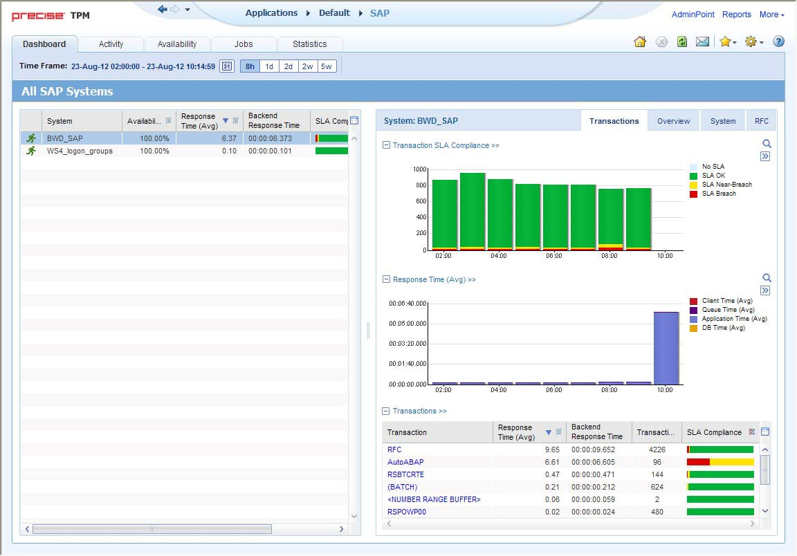
The following figure describes the common key elements in the Activity tab and what happens when you drill down to a specific entity.
Figure 1 Typical Precise for SAP tab structure
About the Precise bar
The Precise bar enables you to keep track of where you have been and provides various controls. The following table describes the function of each of the toolbar buttons.
Table 2 Precise bar functions
| Button | Name | Description |
|---|---|---|
 | Back | During a work session, keeps track of where you have navigated to. The Back button enables you to navigate between previously visited views. The Back control displays your previous view. |
 | Forward | Enables you to navigate to the next view. This button is only enabled if you clicked Back or if you chose a history option. |
 | Stop | Stops a request for information from the server. |
 | Refresh | Updates the data currently displayed. |
 | Favorites | Enables you to add or remove favorites in your Favorites list. |
 | Send | Opens a new email message in your email program with the link to the current application in context. |
 | Home | Navigates to the highest level entity (stays in the same Tier, tab, or view). The time frame settings remain the same. |
 | Help | Opens the online help in context. |
 | Settings | Lets you configure various program settings. |
 | AdminPoint | Launches Precise AdminPoint. |
About the Main area
The Main area displays general information on the selected instance or entity, in context (the entity that is described in the Tab Heading). The structure of this area depends on the selected entity and tab. For example, some views show two overtime graphs, displayed side-by-side, describing two data series.
The View Control drop-down menu allows you to choose different view options. You can access this menu by clicking the arrow icon.
In some tabs, you can filter the contents of the view by clicking the Filter button. See “Filtering data” on page 19.
About the Association area
The Association area lists entities that have similar attributes, and that are related to the selected entity named in the Tab heading. Besides the Tab bar, the Association area is the main navigation tool. It enables you to drill down from one entity to related entities (usually of a different type).
The entities displayed in this area depend on the selected tab and the selected entity. The same entity may be displayed in several tabs, with different data displayed for each one. For example, it is possible to view performance information on Application servers, transactions, etc., in the Activity tab, while in the Availability tab it is only possible to view information on entities that have availability data collected for them, such as Application Servers.
The Association control, accessed by the arrow icon, allows you to associate with different entities. The last option, More..., opens a dialog box that lets you carry out additional operations, such as to view additional associations, change the sort order, or control the number of returned rows.
The information displayed in the Association area is arranged in a tabular format. Each row in the table represents an entity, and each column describes an attribute of the entity, such as text or a graph. It is possible to change the sort order of the entities in the table by clicking a column title.
The Association tabs located above the table let you display different sets of attributes for the entities displayed in the table. The Association tabs are entity-dependent. For some entities, no tabs are displayed. Selecting a tab does not change the list of entities displayed in the table—it only changes which attributes are displayed.
A numeric column can optionally display a graph, and at times, it can display a stacked bar graph as well (where the combined length corresponds to the numeric value of the column). Switching to a graph view in these columns, offers some level of breakdown to the information displayed in the column.
The following icons are used to indicate which format information is displayed.
Table 3 Changing the format in which information is displayed
| Icon | Description |
|---|---|
 | Display the information in numerical format. |
 | Display the information in a bar graph. |
 | Display the information as a stacked bar graph. |
 | Display the information in percentage format. |
The Association area lets you drill down to another entity by clicking a row. The information displayed in both the Main area and the Association area will change to reflect your selection. See “Filtering data” on page 19 and “Associating entities with data that meets specific criteria” on page 19.
About drilling down in context
The term “in-context” means that you can display additional information on a selected item by drilling down to another tab or view. The filter settings you defined (for example, the selected time you chose) and the entity you selected are carried over to the other view or tab, to allow you to continue analyzing your subject from a different perspective. This concept takes on slightly different meanings depending upon where you are attempting to drill down in context from.
For example, when viewing information on a problematic metric in Alerts, you can switch to Precise for SAP to view additional information and continue your investigation.
Alternatively, when viewing information on an instance in the Dashboard tab, you can click on a link in the Instance Details area (right pane) to view additional information on the related tab, in context to your original selection.
In short, the information displayed when drilling down in context is always related to your original selection’s settings.
How a drilldown affects the Tab heading
The Tab heading displays the name of the currently selected entity on this screen. When you drill down to a new entity in the Association area, the Tab heading changes to reflect the name of the newly selected entity.
About configuring Precise for SAP settings
The following settings allow you to control the appearance and behavior of the user interface. They can be configured from the Settings menu on the Precise bar:
- Mapping settings
- Locale settings
- Display settings
- Time Frame settings
Configuring Mapping and Locale settings
Precise for SAP provides performance and utilization information on your SAP system. You can view this data according to your company’s organization structure and locale’s by configuring the relevant Mapping and Locale settings.
For more information, see the Installing SAP Tier Collectors section in the Precise Installation Guide.
Configuring Display settings
In general, when you drill down to an entity, the system automatically opens with a default view or tab selected. You may change to a different view or tab setting to view additional information. If you then switch to a different entity, the system will automatically switch back to the default view and tab selection. If you want to maintain a sticky tab or view selection, meaning that your selected tab or view setting is maintained even if you switch to a different entity, you can set this option in the Settings menu in the Precise bar.
To configure the Display settings
- Choose Display Settings from the Settings menu in the Precise bar.
- In the Display Settings dialog box, select the Maintain the selected tab or view when switching entities option.
Configuring Time Frame settings
You can determine the resolution of the data that is displayed in the overtime graphs using the Time Frame Settings dialog box. By using this dialog box you can define the default time frame to display.
Tasks common to all tabs
The following tasks are commonly performed in most tabs:
- Switching to a different tab
- Selecting a time frame
- Selecting a SAP system to analyze
- Selecting which clients to analyze
- About capacity graphs
- Filtering data
- Associating entities with data that meets specific criteria
- Focusing on information in overtime graphs
- Sending an email message
- Adding, viewing, and deleting Favorites
- Determining which table columns to display
- Copying data to the clipboard
- Exporting to the Precise Custom Portal
Switching to a different tab
You can easily switch between the different tabs using the Tab Selection bar. When you start your Precise product, the Dashboard tab opens by default. For other Precise products, another tab will open by default. The button of the selected tab is displayed in orange.
To select a tab, click a button on the Tab Selection bar to display information on the selected entity in a different tab.
Selecting a time frame
You can configure Precise for SAP to display transaction performance data for a specific time frame using the predefined time frame options or calendar icons.
Selecting a predefined time frame from the toolbar displays transaction performance data for the selected time period up to the current time. See “Selecting a predefined time frame from the Precise for SAP toolbar” on page 18.
Selecting the time frame using the calendar icon, you can choose to define a time range independent of the current time, or to define a time range up to the current time. See “Selecting a time frame using the calendar icon” on page 18. The predefined time frame options are:
- Last 8 hours (8h) (default)
- Last 1 day (1d)
- Last 2 days (2d)
- Last 2 weeks (2w)
- Last 5 weeks (5w)
The time frame selected affects all information displayed in Precise for SAP. Only data that falls within the selected time frame is shown in these areas.
Selecting a predefined time frame from the Precise for SAP toolbar
To select a predefined time frame, from the Precise for SAP toolbar, select one of the predefined time frames.
Selecting a time frame using the calendar icon
To select a time frame
- Click the calendar icon. In the dialog box that is displayed perform one of the following:
- To define a time frame independent from the current time, select the ‘Time Range’ option and select the Start and End dates and times.
- To define a time frame up to the current time, select the ‘Last’ option and enter the desired time frame.
- To use one of the three previously used time frames, select the ‘Recently used’ option and from the drop- down menu select the desired time frame.
- To use a previously saved time frame, select Use a previously saved time frame and from the drop-down menu select the desired time frame.
- To save your settings for future access, select Save these definitions for future use as: and enter a name in the corresponding field.
- Click OK.
Selecting a SAP system to analyze
You can select the system that you want to analyze in more detail using the System selector.
In most of the tabs (with the exception of the Dashboard tab) it is possible to investigate one system only. The System Selector enables you to choose which system you want to investigate from a list of systems belonging to the selected application. When you choose a different system to study, the information displayed in the tab changes accordingly to display relevant information on the selected system.
Selecting which clients to analyze
The Client selector contains a list of all SAP clients that were configured in the selected system. You can choose to filter out and view information on a specific client’s activities by selecting it from the Client Selector list or choose All Clients to view information on the activities of all SAP clients configured in the selected system.
About capacity graphs
The capacity graph shows how a specific counter (CPU, Load, or Response Time) reacted after an increase in the number of active users or connected users, in the specified system. The capacity graph plots different counters along its x and y axes. A plot on the graph in position (x, y) indicates a sample of these two counters. A best-fit line, representing a linear approximation of the point sampled is also displayed.
Filtering data
You can focus on specific contents of all tabs (except for the Dashboard tab) by showing a subset of the information. This shows the contribution of entities such as programs and users.
You can define flexible selection criteria in the Filter Dialog Box. To open the dialog box, you need to click the Filter Off icon next to the Time Frame selector. Filter On or Filter Off indicates the current state of the filtering mechanism. Filter Off means all information is shown; Filter On means a subset of information is shown.
When you apply your selections in the Filter dialog box, the information displayed in both the Main area and the Association area is modified to reflect your selections. Also, the filtering continues to apply when you drill down to associated entities.
You can enter multiple criteria, in which case each criterion is applied using the logical AND operator.
To filter data
- Click Filter is Off/Filter is On.
- In the Filter dialog box, do the following for each entity you want to filter:
- From the left drop-down list, select an entity.
- From the middle drop-down list, select an operator, such as, Like, <>, Not Like, In, Not In.
- In the text box, type the criteria (case-sensitive) for the selected entity. If you select the operator Like or Not Like, you can use the % wildcard character to represent zero or more characters, and the _ wildcard character to represent exactly one character. If you select the operator In or Not In, type a comma to separate values.
- Click OK.
Associating entities with data that meets specific criteria
You can associate the displayed entity with specific data to focus your analysis.
The criteria no longer apply when you drill down to another entity.
To associate entities with data that meets specific criteria
- Click the arrow located to the left of the Association controls and select More... (applies to Current and Objects tabs only).
- In the Associate With dialog box, on the Entries tab, select the entity you want to associate data with from the Populate table with list.
- In the Sort entries by list, determine according to which criteria you want the information to be sorted and in which order.
- From the Display top list, select the number of rows to display.
- On the Criteria tab, do the following for each entity you want to associate data with:
- From the left drop-down list, select an entity.
- From the middle drop-down list, select an operator, such as, Like, <>, Not Like, In, Not In.
- In the text box, type the criteria (case-sensitive) for the selected entity. If you select the operator Like or Not Like, you can use the % wildcard character to represent zero or more characters, and the _ wildcard character to represent exactly one character. If you select the operator In or Not In, type a comma to separate values.
- Click OK.
Focusing on information in overtime graphs
Some entities display an overtime graph. The overtime graph displays entity statistics over a specified time period. Depending on the number of points displayed in the graph, you may need to zoom in or out. The text displayed on the x-axis varies according to the time frame. If there is a year or day change, x-axis labels will display accordingly.
To focus on information in overtime graphs, select the desired time frame on the overtime graph, click and drag the left or right handle to increase or decrease the time range. The small zoom (spyglass) icon will display on the upper right of the selected time range, and above the overtime graph legend. Click the zoom icon to zoom in according to the selected time frame.
Sending an email message
You can send an email message to one or more recipients from the Precise toolbar. The default subject for the message will be “Link to a Precise application”.
The email will include a link to the Precise product in the current context (time frame and selected entries).
To send an email message
- Click the email icon on the Precise toolbar. The default email program opens.
- Fill in the required fields and click Send.
Adding, viewing, and deleting Favorites
The Favorites feature allows you to save a specific location in your application and to retrieve the same location later without having to navigate to it.
About the Favorites feature
The new Favorites feature includes the following options:
- Relative Time Frame. Saving relative timeframe instead of static date. For example, saving the last 7 days will always display the last 7 days, depending on the day entered.
- One click to specific location. Once you open Precise by launching a saved Favorite item, you will not have to enter a login credential nor click the login button.
- IE Favorites support. Adding a new Favorite item in Precise will also add it to the IE Favorites menu.
- Auto Complete. The Favorites dialog includes a new combo box which supports AutoComplete.
- Auto Naming. The Favorites dialog generates item names based on the current location.
UI description
A Favorites menu has been added to the Precise bar in each product including StartPoint.
An Add/Delete Favorites option under the Favorites menu allows you to save the current location or delete an existing one.
To add a new Favorite location
- On the Add/Delete Favorites dialog box, enter the name of the new Favorites entry.
- Click Add. The dialog box is closed and the new Favorite is added to the list.
To view a Favorites location
- On the Precise bar, click Favorites.
- Select the Favorites location you want to view.
To delete an existing Favorite location
- On the Add/Delete Favorites dialog box, select the Favorite location to be deleted.
Click Delete. The dialog box closes and the selected Favorite is deleted from the list.
The favorite address is displayed in the Address field and cannot be edited.
Determining which table columns to display
Tables are used to display information about the set of related entities in the Main and Association areas. It is possible to determine which columns to display in the Association area tables.
To determine which columns to display in the Association area
- Click the Table icon on the upper right-hand side of a table and select Column Chooser.
- In the Table columns dialog box, click the arrows to move the names of the columns that you want to display to the Visible box and the ones that you do not want to display to the Invisible box.
- Click OK.
Copying data to the clipboard
At times you may want to save data displayed in the table area in a Microsoft Excel spreadsheet for further analysis or save an image of a graph to the clipboard.
To copy data displayed in the Association area to the clipboard, click the Table icon on the upper right-hand side of a table and select Copy to clipboard. The table can be pasted into Microsoft Excel or as an HTML file.
To copy a graph to the clipboard, right-click a graph and choose Copy to clipboard. You can now paste the image into any application that works with the clipboard.
Exporting to the Precise Custom Portal
The Export to the Precise Custom Portal Portlet feature enables you to export the view of the chosen table or graph and generate a portlet with that view in the Precise Custom Portal, so that it will provide you with another way of monitoring your application.
Prerequisites
To be able to use this feature, you need to have the following rights in Precise:
- View permissions to all Tiers in the application
If you do not have sufficient rights, you will get an error message when trying to execute this feature.
Exporting the information
You can either export a table view or a graph view.
The name field has the following restrictions: maximum 100 characters.
To export a table view
- Click the Column Chooser icon.
- Select Export to the Precise Custom Portal Portlet.
- Insert a name in the name field that clearly describes the table view.
- Click OK.
To export a graph view
- Right-click the graph.
- Select Export to the Precise Custom Portal Portlet.
- Insert a name in the name field that clearly describes the graph view.
- Click OK.
About the counters in Precise for SAP
Counters help you analyze your systems activities and batch processes. Information on the following counters is displayed in the Activity and Batches tabs:
- Response Time
- Application Time
- DB Time
- Requests
- Time per Request
- Average Server Buffer Ratio
- Memory Resources
About response time counters
Response time counters help determine if an application's time is proportional to the amount of time it should be spending for client, queue, application and database processing.
The following table describes the information displayed by the response time counters.
Table 4 Response time counters
| Counter | Description |
|---|---|
| Client time | If working in a LAN, client time should be a very small portion of total SAP response time. |
| Queue time | Should be a very small portion (less than 1%) of the total SAP response time. When this value is high, other long-running transactions or batch programs prohibit proper throughput, or not enough work processes are available. |
| Application time | Includes load time and should be no more than 60% of total SAP response time. When this value is high, the CPU is slowed down, there are SAP memory shortages or the program takes an excessive amount of time for load, queue or ABAP/4 application processing. |
| DB time | Should be approximately 40% of total SAP response time. |
About application time counters
Application time counters help you determine which application time component constitutes a performance bottleneck. The following table describes the information displayed by the application time counters.
Table 5 Application time counters
| Counter | Description |
|---|---|
| Load time | Should be no more than 10% of the application’s total response time. If this value exceeds 10%, this indicates that the SAP System is spending too much time loading the application. Check the Memory Resources counter to determine if there are any SAP memory shortages. If it appears that the CPU or memory resources are sufficient for the application’s processing, check for the following actions:
|
| Enqueue time | Should constitute a small percentage of the application time. When enqueue time is high, check or perform the following actions:
|
| Roll-wait time | The number of seconds that may be required to wait during roll-in of context information for dialog steps. The number of seconds required to transfer GUI control-related information to the front-end solution is also included. During processing, a program may result in a roll-out while waiting for other processing to take place. The process of roll-out and roll-in (in this case) is usually a change of memory pointers, and roll-wait time is minimal. In SAP 4.6 and higher, several communication steps, called round trips, can occur between the application servers and the front-end system. During the round trip, the application server transfers GUI control-related information to the front-end system. The work process is rolled-out and this time is recorded under roll-wait time. Network and front-end time are included as part of roll-wait time, but only as it applies to the control-related information transferred between the application server and the front-end system during the execution of the dialog step. Network time associated with the first request and the last request is therefore not included in roll-wait time. Roll-wait time should be very low. When high, perform the following steps:
|
| Process time | Should constitute 50-60% of the application’s total SAP response time. When this percentage is higher than it should be, system or SAP memory resources are an issue or the application is spending too much time in application logic. Take the following steps:
|
About DB time counters
DB time counters identify whether database response time is attributed to sequential reads, direct reads or changes by comparing their times.
DB time counters refer to the Time Per Request section to determine if response times fall within acceptable performance ratings.
When database time is attributed to sequential reads or direct reads, see the Application Buffer Ratio and investigate whether buffering techniques are optimized for read requests.
The following table describes the information displayed by the DB counters.
Table 6 DB time counters
| Counter | Description |
|---|---|
| Sequential Reads | The response time for logical database requests associated with sequential reads (for example, "select * from ..." ABAP/4 statements). |
| Direct Reads | The response time for logical database requests associated with direct reads (for example, "select single ..." ABAP/4 statements). |
| Changes | The response time for logical database requests associated with database inserts, updates and deletes. |
About requests counters
Requests counters show the volume of database read requests and change requests. The following table describes the information displayed by the Requests counters.
Table 7 Requests counters
| Counter | Description |
|---|---|
| Sequential Reads | The number of logical database requests associated with sequential reads (for example, "select * from ..." ABAP/4 statements). |
| Direct Reads | The number of logical database requests associated with direct reads (for example, "select single ..." ABAP/4 statements). |
| Changes | The number of logical database requests associated with database inserts, updates and deletes. |
See “About DB time counters” on page 24 and “About average server buffer ratio” on page 25.
About time per request counters
Time per request counters identify when database requests do not fall within their performance boundaries. The following table describes the information displayed by the Times per request counters.
Table 8 Time per request counters
| Counter | Description |
|---|---|
| Sequential Reads | The response time, per request, for logical database requests associated with sequential reads (for example, "select * from ..." ABAP/4 statements). |
| Direct Reads | The response time, per request, for logical database requests associated with direct reads (for example, "select single ..." ABAP/4 statements). |
| Changes | The response time, per request, for logical database requests associated with database inserts, updates and deletes. |
When analyzing these counters, keep in mind the following issues:
- Sequential reads should be less than 40 milliseconds per request.
- Direct read requests should be less than 10 milliseconds per request.
- Change requests are expected to be greater than 25 milliseconds per request.
- When per request times are not within their expected performance boundaries:
- Use the DB Time section to determine the importance of the types of read or change requests in question, with respect to the overall response time.
- Use the Requests section to understand the request volume involved in read and change requests.
- When sequential reads or direct reads are performing poorly, see the Application Server Buffer Ratio section to investigate whether buffering techniques are optimized for read requests.
- When changes or reads are performing poorly and your Application Server Buffer ratio appears normal, but the number of returned rows appears unacceptable, the database is likely the source of the problem and should be examined for additional indexes or other causes.
About average server buffer ratio
The average server buffer ratio illustrates the degree of optimization related to application server buffering techniques, which optimize performance for database requests by avoiding the need to transfer read requests to the database server.
The following table describes the information displayed by the average server buffer ratio.
Table 9 Average server buffer ratio
| Counter | Description |
|---|---|
| Sequential Reads | The percentage of time sequential read requests were handled by the application server, instead of the database server. Sequential read requests refer to logical database requests associated with sequential reads (for example, "select * from ..." ABAP/4 statements). |
| Direct Reads | The percentage of time direct read requests were handled by the application server, instead of the database server. Direct read requests refer to logical database requests associated with direct reads (for example, "select single ..." ABAP/4 statements). |
Keep in mind the following issues when analyzing these counters:
- App Server Buffer Ratios should typically be 90% or greater. The higher the percentage indicates that fewer read requests are transferred to the database server and performance is optimized.
- If this percentage is low, determine the importance of the App Server Buffer Ratio to your transaction's database performance:
- Check the DB Time section of this view to determine if database response time is mostly attributed to reads (sequential and direct) or changes.
- Database time attributed mostly to changes suggests that the Buffer Ratio is not an important factor to overall response time—this is because changes are always transferred to the database server.
- When database time is influenced by reads, the buffer ratio is likely to impact overall database time. Buffer usage, for example, can reduce response time for database reads by as much as 10 times.
- Consider implementing 1 of these 3 buffering techniques to increase read performance and reduce load on the database server.
- Buffer data as context in the shared memory buffer.
- Buffer data in a table using a generic key or single record buffer.
- Buffer data using an internal table of a function module.
- Note the following regarding buffering techniques:
- Restrict buffering techniques to read-only data as much as possible to minimize buffer synchronization across application servers.
- When selecting a buffering technique, take data size requirements into consideration. An instance typically has about 50 MB of data in the shared memory and buffers, whereas, information stored in internal tables should not exceed 5 MB.
- Buffered tables take much more effort to change than non-buffered tables. Therefore, restrict buffered tables to read-only data stored in customizing tables or small tables.
About memory resources
Memory resources determine if an application is receiving a sufficient amount of SAP application server memory resources.
The following table shows which counters are included in the Memory resources.
Table 10 Memory resources
| Counter | Description |
|---|---|
| Private Mode | Private mode conditions should not occur. When private mode conditions occur, the SAP application server's shared memory is insufficient to meet the demands of the application, and the following occurs:
|
| Extended Memory | To determine memory shortage impact on an application's response time, do the following:
|
Launching your Precise product from StartPoint
Precise is a Web-based application. You can access the Precise user interface using the Internet Explorer browser, version 6.0, or later. The syntax of the Precise URL address is http://<server>:<port>,where <server> refers to the Precise FocalPoint server and <port> refers to the port number used by the GUI Web server. By default, the port number is 20790. For example: http://beantown:20790.
This URL provides secure access to the StartPoint using authorized roles. From here, you can launch all Precise products. It gives you a quick overview of the status of your environments and access to the AdminPoint, where you can perform various management tasks (see the Precise Administration Guide for details).
You must have local administrator privileges on the server where the StartPoint is running.
To launch your product using StartPoint
- Type the address of the StartPoint user interface into the Address bar of your browser and click Enter. The Precise login page opens. The login page provides secure access to Precise and to your specific product.
- Specify your authorized role name and password. By default, both role name and password are admin. For more information about role names, see the Precise Administration Guide.
- Click Login. The StartPoint page opens. This is the Precise home page.
- On the Product Selection bar, from the drop-down list, select the product you want to launch.