SQL Query Tuner's methodology grew out of the impossible predicament presented by the defacto method of database tuning. The standard method was trying to collect 100% of the statistics 100% of the time. Trying to collect all the statistics as fast as possible ends up putting load on the monitored database and creating problems. Stories of problems created by database monitoring products abound in the industry. In order to avoid putting load on the target database, performance monitoring tools have to collect less often as a compromise. Oracle compromised in 10g with AWR (their automated performance data collector), only running it once an hour because of the performance impact. Not only is the impact on the monitored target high, but the amount of data collected is staggering, but the worst problem of all though, is the impossibility of correlating statistics with the sessions and SQL that created the problems or suffered the consequences.
The solution to collecting performance data required letting go of the old problematic paradigm of trying to collect as many performance counters possible as often as we could and instead freeing ourselves with the simple approach of sampling session state. Session state includes what the session is, what its state is (active, waiting, and if waiting, what it is waiting on) and what SQL it is running. The session state method was officially packaged by Oracle in 10g when they introduced Active Session History (ASH). ASH is an automated collection of session state sampling. The rich robust data from ASH in its raw form is difficult to read and interpret. The solution for this was Average Active Sessions (AAS). AAS is a single powerful metric which measures the load on the database based on the ASH data. AAS data provided the perfect road map for what data to drill into. The main drill downs are "top SQL", "top session", "top event", and "top objects".
Other aggregations are possible based on the different dimensions in the ASH data.
Tuning Example
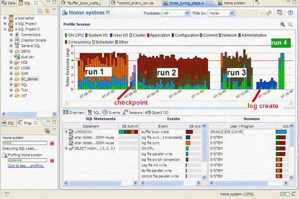
Here is an example screen shot of the same batch job being run four times. Between each run performance modifications are made based on what was seen in the in the profiling load chart:
Run:
- In run 1, the log file sync event is the primary bottleneck. To correct this, we moved the log files to a faster device. (You can see the checkpoint activity just after run 1 where we moved the log files.)
- In run 2, the buffer busy wait event is the primary bottleneck. To correct this, we moved the table from a normal tablespace to an Automatic Segment Space Managed tablespace.
- In run 3 the log file switch (checkpoint incomplete) event is the primary bottleneck. To correct this, we increased the size of the log files. (You can see the IO time spent creating the new redo logs just after run 3.)
- The run time of run 4 is the shortest and all the time is spent on the CPU which was our goal, take advantage of all the processors and run the batch job as quickly as possible.
To view an explanation of the event, hover over the even name in the Event section.
Conclusion
With the load chart we can quickly and easily identify the bottlenecks in the database, take corrective actions, and see the results. In the first run, almost all the time is spent waiting, in the second run we eliminated a bottleneck but we actually spent more time - the bottleneck was worse. Sometime this happens as eliminating one bottleneck causes great contention on the next bottleneck. (You can see the width of the run, the time it ran, is wider in run 2). By the third run, we are using more CPU and the run time is faster and finally by the 4th run all the time spent is on CPU, no waiting, and the run is the fastest by far.